Source: View original notebook on GitHub
Category: Machine Learning / Learn ML
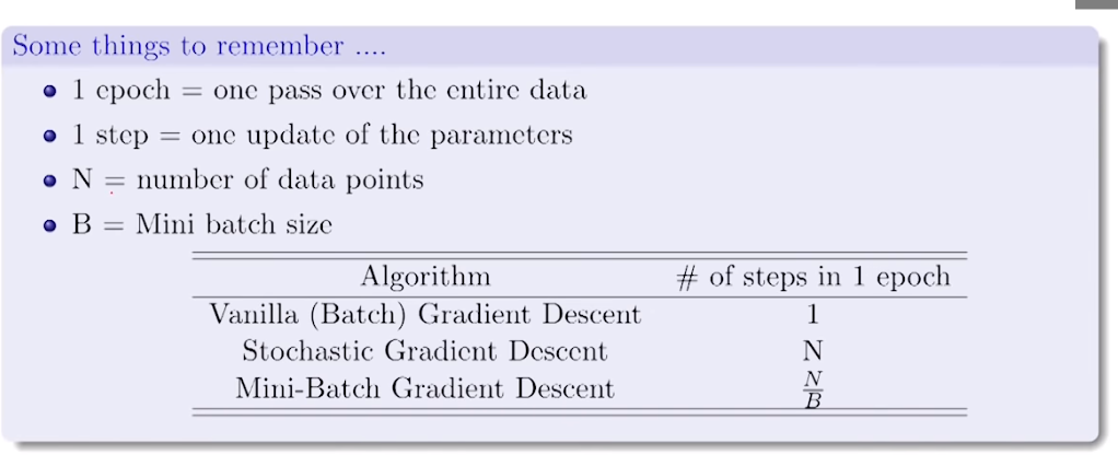
Gradient descent we learned till now is Batch(complete sample) Gradient descent
Earlier in Gradient descent algorithm we were making one update(taking one step toward minima) to our thetas by going through all the samples of our data, suppose if we have millions of sample points then to make a single update we go over the complete sample, it is time consuming.
but why were we doing that !! beacause that was the right thing to do !! as we derived that using error function, so yes that should have happened.
def gradient(X,Y,theta):
    grad = np.zeros(2)
    hx = theta[0] + theta[1]*X
    grad[0] = np.sum(hx-Y)
    grad[1] = np.sum((hx-Y)*X)
    return grad

# code similar to we written in 3rd notebook for univarate gradient descent
def batch_gradientDescent(X,Y,learning_rate=0.0001):
    theta = np.zeros(2)
    itr = 0
    max_itr = 1000

    while itr<max_itr:
        # calulate the gradent over complete sample
        grad = gradient(X,Y,theta)
        # updating after it
        theta[0] = theta[0] - learning_rate * grad[0] # grad 0 is d(cost) / d(theta 0)
        theta[1] = theta[1] - learning_rate * grad[1] # grad 1 is d(cost) / d(theta 1)
        itr += 1

    return theta
Stochastic(Approximation) Gradient Descent
now instead of going through the complete sample and then making a update, we go for an approximation,and  update our theta for each and every sample points .
what will happen??
    - now there is no guarantee that each update will decrease our loss , or we move toward the minima !! why? !! beacuse now every single sample point is trying to push the parameters(theta) in the direction more favourable to it, without being thinking how will it affect other points.

    - so for now  in one single step of moving toward minima , we are doing oscillation before taking a single step.
This is called stochastic gradient Descent.
def gradient(X,Y,theta):
    grad = np.zeros(2)
    hx = theta[0] + theta[1]*X
    grad[0] = np.sum(hx-Y)
    grad[1] = np.sum((hx-Y)*X)
    return grad

def stochastic_gradientDescent(X,Y,learning_rate=0.0001):
    theta = np.zeros(2)
    epoch = 0 # epoch means iteration
    max_epoch = 1000

    while epoch<max_epoch:
        for each_sample in range(X.shape[0]):
            grad = gradient(X[each_sample],Y[each_sample],theta)
            # updating for each example after it
            theta[0] = theta[0] - learning_rate * grad[0] # grad 0 is d(cost) / d(theta 0)
            theta[1] = theta[1] - learning_rate * grad[1] # grad 1 is d(cost) / d(theta 1)
        epoch += 1

    return theta
Mini-Batch Gradient Descent
we can do better than stochastic by making an update to parameters in some batches(dividing our sample into some batches) instead of doing that at every single sample point, this way we would have less oscillations than stochastic ,but we will have the trajectory of this mini-batch contained inside the stochastic (because of less oscillations).


so we can say that if batch size is one , mini-batch is similar to stochastic Gradient Descent.
def gradient(X,Y,theta):
    grad = np.zeros(2)
    hx = theta[0] + theta[1]*X
    grad[0] = np.sum(hx-Y)
    grad[1] = np.sum((hx-Y)*X)
    return grad

def mini_batch_gradientDescent(X,Y,learning_rate=0.0001,batch_size = 4):
    theta = np.zeros(2)
    epoch = 0
    max_epoch = 1000

    while epoch<max_epoch:
        grad = np.zeros(2)
        for each_sample in range(X.shape[0]):
            # calculating graient over the current batch
            grad += gradient(X[each_sample],Y[each_sample],theta)

            # updating for each batch only
            if (each_sample % batch_size) == 0 :
                theta[0] = theta[0] - learning_rate * grad[0] # grad 0 is d(cost) / d(theta 0)
                theta[1] = theta[1] - learning_rate * grad[1] # grad 1 is d(cost) / d(theta 1)
                grad = (0,0) # resetting gradient

        epoch += 1

    return theta