
Source: View original notebook on GitHub
Category: Machine Learning / Learn ML
Linear Regression
Objective of supervised Learning
- we want to generate a function or hypothesis from training data using some algorithm and then from the function we can predict the output for our test data.

-
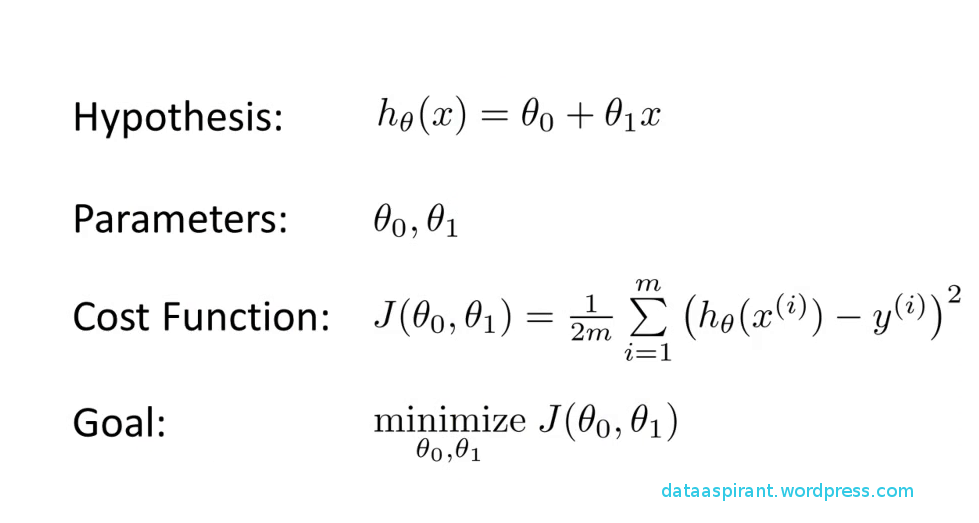
Objective of linear Regression
- let the function be a type of linear function i.e for vector x(x1,x2,x3,.....,xn) we have function as
    - f(x) = a(x1) + b(x2)+ c(x3)...............+ alpha(xn) + constant

- now we have to chose (a,b,c,d,.......,alpha) in such a way we predict as closely as possible to real outcome
- for that we defined our error/cost function as in figure and our goal is to minimize it : -
- here let data be univariate
- cost function is convex function so local minima is global minima.
Method 1 (minimizing error function equating differentiation to 0 and finding slope and intercept by solving two equations)
-  using formulas done by the calculating  slope and intercept value
-  for slope and intercept we minimize the error function using differentiation
    - slope = cov(x,y)/cov(x,x)
    - intercept = E(y) - slope*E(x)
cov(x,y) = E(xy) - E(x)E(y)
import numpy as np
import pandas as pd
import matplotlib.pyplot as plt
X = pd.read_csv('Datasets/linearX.csv')
Y = pd.read_csv('Datasets/linearY.csv')
X = X.values
Y = Y.values
X.shape
Output:
(99, 1)
Y.shape
Output:
(99, 1)
Visualization and Normalization/Standarization
%matplotlib inline
plt.style.use('seaborn') #just changing graph style
# normalization/standarization of Data
X  = (X-np.mean(X))/np.std(X)
plt.scatter(X,Y,marker='*',s=100)

Output:
<matplotlib.collections.PathCollection at 0x11b8fef0>
# using method 1

# theta1
theta1_num = np.mean(X*Y) - np.mean(X)*np.mean(Y)
theta1_den = np.mean(X*X) - np.mean(X)*np.mean(X)
theta1 = theta1_num / theta1_den

# theta0
theta0 = np.mean(Y) - theta1*np.mean(X)

theta1,theta0
Output:
(0.0013579397686593838, 0.9966341414141414)
plt.scatter(X,Y,c='blue',marker='*',s=100)
plt.plot(X,theta0+theta1*X, 'r',lw=2)

Output:
[<matplotlib.lines.Line2D at 0x11cef3f0>]
from sklearn.metrics import r2_score
r2_score(Y,theta0 + theta1*X)
Output:
0.43818504557919435
Method 2 (gradient descent) (Important)
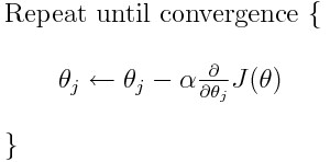
what is Gradient Descent?
an algorithm to iteratively finding out the minimum value of a convex function by updating parameters in such a way that we move toward the minimum point .
Gradient descent is a first-order iterative optimization algorithm for finding the minimum of a function. To find a local minimum of a function using gradient descent, one takes steps proportional to the negative of the gradient(slope) (or approximate gradient) of the function at the current point.
X.shape
Output:
(99, 1)
Y.shape
Output:
(99, 1)
steps of gradient descent
- start from random point (theta0,theta1)
- update thetas using gradient
- move toward minimum till convergence
convergence criteria
- fixed number of iteration
- change in error < small number(0.001) --> good criteria than above
# lets do for univariate data
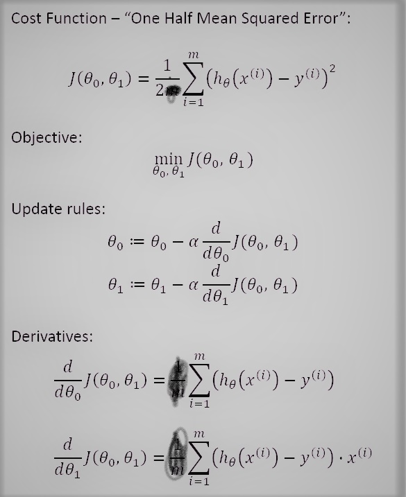
# my cost function or error is (1/2)*(sigma [(hx-yi)**2] )
# see i didn't use m here(or anywhere) since that was just to make calculation simple ,i dont want that!!! :)
def hypothesis(X,theta):
    return theta[0] + theta[1]*X
def gradient(X,Y,theta):

    grad = np.zeros(2)
    hx = hypothesis(X,theta)

    grad[0] = np.sum(hx-Y)
    grad[1] = np.sum((hx-Y)*X)

    return grad


def error(X,Y,theta):
    hx = hypothesis(X,theta)
    return (1/2)*(np.sum((hx-Y)**2))
def gradientDescent(X,Y,learning_rate=0.0001):

    # starting- point ()
    theta = np.zeros(2)

    # using fixed number of iteration
    itr = 0
    max_itr = 1000

    error_list = []
    while itr<max_itr:
        grad = gradient(X,Y,theta)
        error_list.append(error(X,Y,theta))
        theta[0] = theta[0] - learning_rate * grad[0] # grad 0 is d(cost) / d(theta 0)
        theta[1] = theta[1] - learning_rate * grad[1] # grad 1 is d(cost) / d(theta 1)

        itr += 1

    return theta,error_list
theta_ans,error_list = gradientDescent(X,Y)
theta_ans
Output:
array([0.99658654, 0.00135787])
# generating testing data
X_test = np.linspace(-2,5,50)
plt.scatter(X,Y, marker = '*',s=100)
plt.plot(X_test, hypothesis(X_test, theta_ans),'r',lw=3)
plt.show()

# plotting error function vs iteration
plt.plot(error_list)
plt.xlim(0,400)
plt.xlabel('NUMBER OF ITERATION ')
plt.ylabel('ERROR')

Output:
Text(0, 0.5, 'ERROR')
def gradientDescent_2(X,Y,learning_rate=0.0001):

    # starting- point ()
    theta = np.array([-3.9,3.9])

    # using change in error being very low
    error_list = []
    error_list.append(error(X,Y,theta))

    # theta_list for plotting trajectory
    theta_list=[]
    while True:
        grad = gradient(X,Y,theta)
        theta_list.append((theta[0],theta[1]))
        theta[0] = theta[0] - learning_rate * grad[0] # grad 0 is d(cost) / d(theta 0)
        theta[1] = theta[1] - learning_rate * grad[1] # grad 1 is d(cost) / d(theta 1)
        error_temp = error(X,Y,theta)
        change = abs(error_list[-1] - error_temp)
        if change < 0.00000000000001:
            break
        error_list.append(error_temp)


    return theta,error_list,theta_list
min_theta, error_list,theta_list = gradientDescent_2(X,Y)
min_theta
Output:
array([0.99663406, 0.001358 ])
plt.scatter(X,Y, marker = '*',s=100)
plt.plot(X_test, hypothesis(X_test, min_theta),'r',lw=3)
plt.show()

plt.plot(error_list)
# plt.xlim(0,len(error_list))

plt.xlabel('NUMBER OF ITERATION ')
plt.ylabel('ERROR')

Output:
Text(0, 0.5, 'ERROR')
Visualizing the error function in 3D space and the trajectory of theta vector
import matplotlib.pyplot as plt
from mpl_toolkits.mplot3d import Axes3D
# importing data

import numpy as np
import pandas as pd

X = pd.read_csv('Datasets/linearX.csv')
Y = pd.read_csv('Datasets/linearY.csv')
X = X.values
Y = Y.values
X  = (X-np.mean(X))/np.std(X)


# creating data for Theta0 and theta1 and computing cost function
T0 = np.linspace(-4,4,X.shape[0])
T1 = np.linspace(-4,4,X.shape[0])

J = np.array([[0 for j in range(X.shape[0])]for i in range(X.shape[0])])
for i in range(X.shape[0]):
    for j in range(X.shape[0]):
        J[i][j] = np.sum((T0[i] + T1[j]*X - Y)**2)
T0,T1 = np.meshgrid(T0,T1)
# creating 3d figure and axes
fig = plt.figure()
ax = fig.gca(projection='3d')

ax.plot_surface(T0,T1,J,cmap = 'coolwarm',alpha=0.7)

theta_list = np.array(theta_list)

# trajectory in black
ax.scatter(theta_list[:,0], theta_list[:,1], error_list,marker='>', c='k')

Output:
<mpl_toolkits.mplot3d.art3d.Path3DCollection at 0x18c9270>
Creating plot, 3D/2D contour,surface, wireframe
fig = plt.figure(figsize=(15,10))

ax = plt.subplot(221,projection='3d')
# trajectory in black
ax.scatter(theta_list[:,0], theta_list[:,1], error_list,marker='>', c='k')
ax = ax.plot_surface(T0,T1,J,cmap = 'coolwarm')


ax1 = plt.subplot(222,projection='3d')
# trajectory in black
ax1.scatter(theta_list[:,0], theta_list[:,1], error_list,marker='>', c='k')
ax1 = ax1.plot_wireframe(T0,T1,J)

ax2 = plt.subplot(223,projection='3d')
# trajectory in black
ax2.scatter(theta_list[:,0], theta_list[:,1], error_list,marker='>', c='k')
ax2 = ax2.contour(T0,T1,J,cmap = 'rainbow')

ax3 = plt.subplot(224)
# trajectory in black
ax3.scatter(theta_list[:,0], theta_list[:,1], error_list,marker='^', c='k')
ax3 = ax3.contour(T0,T1,J,cmap = 'rainbow')

Gradient Descent algo in sklearn
import numpy as np
import pandas as pd
import matplotlib.pyplot as plt
X = pd.read_csv('Datasets/linearX.csv')
Y = pd.read_csv('Datasets/linearY.csv')
from sklearn.linear_model import LinearRegression
from sklearn.model_selection import train_test_split
X_train,X_test,Y_train,Y_test = train_test_split(X,Y,test_size=0.2)
lr_model = LinearRegression(normalize=True)
lr_model.fit(X_train,Y_train)
Output:
LinearRegression(copy_X=True, fit_intercept=True, n_jobs=None, normalize=True)
slope = lr_model.coef_
intercept = lr_model.intercept_
slope,intercept
Output:
(array([[0.00078001]]), array([0.99038226]))
model.score(X_test, Y_test) # figuring out how good is the model
Output:
0.4855894020818986
or can find out using r2_score() of sklearn.metrics
from sklearn.metrics import r2_score
r2_score(Y_test, lr_model.predict(X_test))
Output:
0.4886661642049145
plt.scatter(X,Y, marker = '*',s=100)
plt.plot(X, slope*X+intercept,'r',lw=3 )
plt.show()
