
Source: View original notebook on GitHub
Category: Machine Learning / Learn ML
Types of Naive Bayes
In Sklearn there are 4 types of Naive Bayes out of which 3 are important :
0. Simple Naive Bayes (covered inside Multinomial in sklearn)
-> learned so far => X is categorical Data => Example : Mushroom dataset
1. Gaussian Naive Bayes
-> X is numerical Data (Real valued Data) => Example : Iris dataset
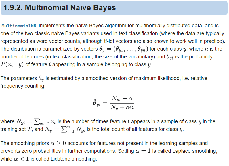
2. Multinomial Naive Bayes
-> X is categorical Data( with each feature having >= two classes )
-> Simple Naive Bayes + Laplace Smoothing(numerator is added with 1 , but denomenator with |V|) => create a vector of unique words occured in training data with its frequency noted. V is number of unique words present in Dataset
-> used in Text/Document classification
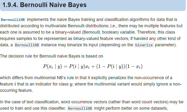
3. Multivariate Bernoulli Naive Bayes
-> X is categorical Data ( with each feature having two classes(binary) )
-> Laplace Smoothing is used here as well.(numerator is added with 1 , but denomenator with 2)
-> There may be multiple features but each one(xi) is assumed to be a binary-valued (Bernoulli, boolean) variable
- The difference is that while MultinomialNB works with occurrence counts, BernoulliNB is designed for binary/boolean features.
- The different Naive Bayes classifiers differ mainly by the assumptions they make regarding the distribution of P(xi|Y=c).
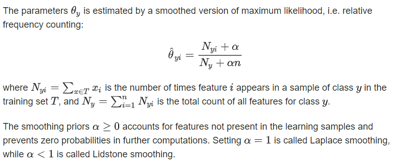
Laplace Smoothing :
Must Read Blog(https://monkeylearn.com/blog/practical-explanation-naive-bayes-classifier)
since likelihood is measures by the product of p(trainingFi==queryFi|c), i = {0,1....} and if one of term become zero(because of no matching of queryFeature to training data fratures) whole product goes to zero hence probabilty becomes zero as well. which is incorrect or say training data have not seen the new data at all.
*Use Laplace/Additive Smoothing* => add 1 to numberator and d to denominator while calcualting each p(fi|c) where d is the |V| and where |V| is the length of dictionary formed using Bag of Words Model over text in a document.
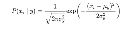
1. Gaussian Naive Bayes
from sklearn.datasets import load_iris()
iris = load_iris()
from sklearn.naive_bayes import GaussianNB
gnb = GaussianNB()
y_pred = gnb.fit(iris.data, iris.target).predict(iris.data)
The likelihood of the features is assumed to be Gaussian:
2. Multinomial Naive Bayes
import numpy as np
X = np.random.randint(5, size=(6, 100)) # 5 because in multinomial each feature have >=2 classes
y = np.array([1, 2, 3, 4, 5, 6])
from sklearn.naive_bayes import MultinomialNB
clf = MultinomialNB(alpha =1.0)
clf.fit(X, y) # alpha is the smoothing parameter
Output:
MultinomialNB(alpha=1.0, class_prior=None, fit_prior=True)
print(X[2:3])
print(clf.predict(X[2:3]))
Output:
[[0 4 0 2 2 3 1 0 0 1 2 0 2 4 2 3 1 0 1 2 2 1 1 3 3 0 1 0 3 1 2 2 3 4 3 3
  2 3 0 4 2 0 0 2 4 4 3 0 3 1 4 0 0 2 0 4 3 2 0 0 0 1 2 4 3 3 4 3 0 4 3 4
  3 0 3 2 4 1 2 4 2 4 1 4 4 3 1 2 0 0 3 3 0 0 3 3 3 3 2 0]]
[3]
y[2]
Output:
3
3. Multivariate Bernoulli Naive Bayes
import numpy as np
X = np.random.randint(2, size=(6, 100)) # values are taken binary only (using 2)
Y = np.array([1, 2, 3, 4, 4, 5])
from sklearn.naive_bayes import BernoulliNB
clf = BernoulliNB()
clf.fit(X, Y)
print(clf.predict(X[2:3]))
Output:
[3]
Key Difference in Multinomial and multivariate bernoulli NB
in multinomial vector formed is <1,2,3,4,1,0,1,2,2,3,3,4,2,3,2,4,3,1,4,2,1,0,2,0,3,0,0,3,2,0,0,3,0,1,2,3> means fequency of ith word is stored ,with |V| being total unique words in documents
in multivariate Bernoulli, vector formed is <1,0,0,0,1,0,1,1,1,0,....> means absence or presence of words in a sentence.