Source: View original notebook on GitHub
Category: Machine Learning / Learn ML

Logistic Regression(`Classification Algorithm`)

Although name has Regression in it but it is a Classification Algorithm
in classification problems we deal with the data which is qualitative or categorical(like eyes color -blue,green,red etc).
values are discrete values, hence are grouped into classes
so in Classification , we have classes , our goal is to predict the class of a new sample or to which class it belongs to.
for that we make a decision boundary to seperate one class data points clusters from other.
in total we have Kc2 boundaries, where k is the number of the number of classes our data have.

Binary Classification

Let for simplicity (for now), we are taking data with two class only hence it is Binary Classification.

Using Logistic Regression for Binary Classification

- since our data have two classes , lets say 0 and 1 , we need to predict 0 and 1 only.

- let our decision Boundary be Linear in nature just like in case of Linear Regression ,written as 
    h(X) = theta[0] + theta[1]*X1 + theta[2]*X2 + ........
    
- but there is one Problem with this function ,its value ranges from (-inf to inf), hence cannt be used here.

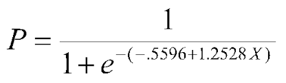
- To solve this Problem we defined a Sigmoid Function as `g(Z) = 1/1+e^(-h(x))`,which always results in values (0,1), both excluded, hence can be used in our Binary Classification.

Visualizing sigmoid Function

import numpy as np
import matplotlib.pyplot as plt

def sigmoid(x):
    return 1 / (1 + np.exp(-x))

x = np.arange(-10,10,0.01)
y = sigmoid(x)

plt.plot(x,y)
plt.yticks(ticks=[0,0.5,1])
plt.grid()
plt.show()

Output

Logistic Regression Intuition

- since in Linear Regression, we got a line h(x), similarly we got it here but also passing it to sigmoid function.
- here we will train our Algorithm that if we got a line and
- if h(x) = (theta.T)*X &gt;=0 ,then we say the points(mostly) lies on one side will belong to Class 1.
- else if h(x)&lt; 0, we got all the remaining points lies on other side will belong to Class 0.

- this is true because all we want is that boundary only.

- according to that if h(x)&gt;=0, then g(h(x)) &gt;=0.5 (see from the graph) else we will have &lt;0.5

- so our hypothesis becomes , if g(h(x))&gt;=0.5 , we will get class 1 ,otherwise clas 0

Conclusion

in conclusion we can say that more the probability,better is the chance it belongs to class 1.

Goal of Logistic Regression

we will write , theta as w
we can say that

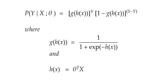
    - P(Y=1|X;w) = g(h(x))
    - P(Y=0|X;w) = 1 - g(h(x))

why? because if g(h(x)) comes out to be greater than 0.5 , there is more chance ,it belongs to class 1.

we can write that down in one line as

that is for one point only, the likelihood that it belongs to a class

Assumption (Samples are Independent from each others)

since we want likelihood of all the INDEPENDENT points , we got it as the product of them , GOAL: - we want to maximize the likelihood that it belongs to same class as it should be.

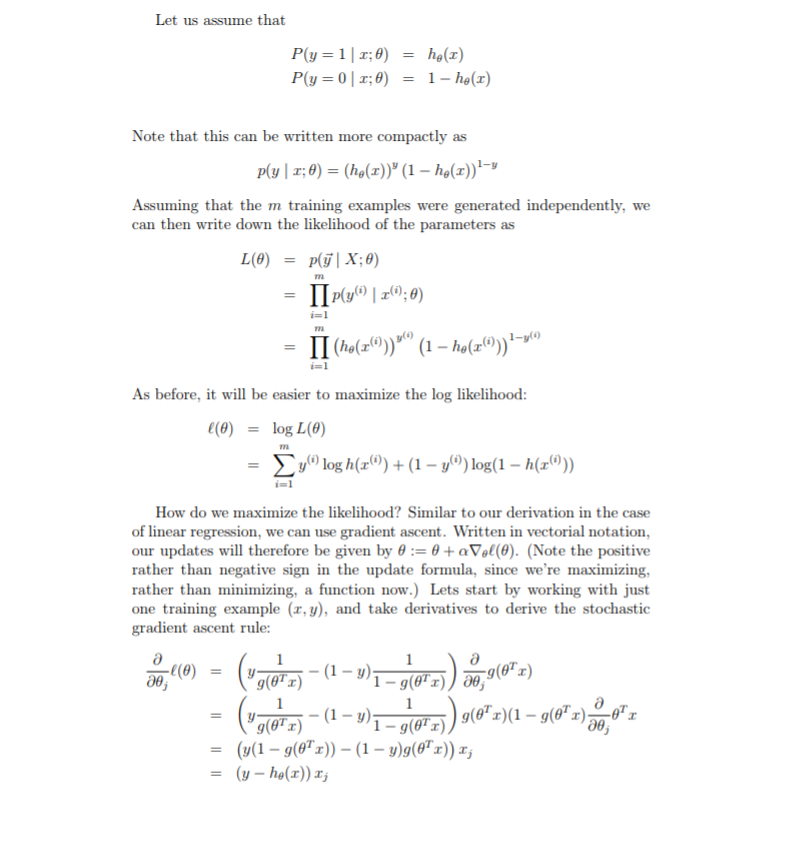
Above, we used the fact that g′(z) = g(z)(1 − g(z)). This therefore gives us the stochastic gradient descent rule
            θj := θj - α(hθ(x(i)-y(i))*x(i)j)

If we compare this to the LMS update rule, we see that it looks identical; but this is not the same algorithm, because hθ(x(i)) is now defined as a non-linear function of θTx(i) .

Nonetheless, it’s a little surprising that we end up with the same update rule for a rather different algorithm and learning problem. Is this coincidence! 

Logistic Regression(Classification Algorithm)